[ER] returns home
in orbitCompleted


- My role
- Data / Backend
- Team
- 6 Seniors
- When
- Sept 2025 - May 2026
Is there a best way to drive a Formula 1 car?
This project was awarded the CSCE Undergraduate Enrichment Fund.

At a glance
A year-long capstone for General Motors where we set out to define “driving styles” amongst F1 drivers.
- Awards: 1st place for the CSCE Undergraduate Enrichment Fund, 1st place at the College of Engineering Expo (CSCE), and an invitation to present at the CSCE Alumni Conference.
- My part: I was the main developer of the scraper, database, and preprocessing pipeline, and made 78 of the team’s 167 commits.
- Scale: 26,692 laps from all 24 races of the 2025 F1 season. Over 18 million telemetry samples, stored as over 36 million database rows.
- Live: f1.elirose.dev
The prompt
Formula 1 teams measure everything about the car, but the driver is still hard to quantify.
Lap time is the metric everyone looks at, but it’s shaped by everything around the driver just as much as the driver themselves. GM asked us to build a tool that digs into what exactly differs amongst drivers, and to do so independent of lap time. It was an interesting challenge, and one that had previously been relatively unexplored in F1 data analytics (see ‘3.2 Related Work’ in our paper).
Capstone at the University of Arkansas is two semesters. In the fall, we were matched with an industry sponsor and designed a solution to the sponsor’s given problem statement. In the spring, we built it. My team of six was sponsored by General Motors, whose data science team mentored us throughout the project’s duration.
My role
I wrote nearly all of data_ingestion/ and the core of data_analysis/.
data_ingestion/├─ scrape.pydownloads every lap├─ postgresql_db.pycreates the 48 tables├─ database_intake.pyvalidates and loads laps├─ psql_index_creation.pyindexes driver and lap└─ query_db.pychecks the loaddata_analysis/├─ cache/│ └─ build_metadata_cache.pylap counts per race├─ query_db.pyfetches one lap├─ race_data.pycleans a race├─ export_library.py(teammate) logs dropped laps└─ kmeans_clustering.py(shared) clusters a racefrontend/(teammate) the dashboardscrape.py and database_intake.py
All 26,692 laps of the 2025 season, loaded into PostgreSQL after three failed overnight runs.
Getting the data in took four tries. The first three overnight loads failed, so I added two safeguards to database_intake.py. Every row is validated against the database’s checks, and the telemetry and metadata row counts are reconciled to confirm both tables match.
The scraper uses FastF1 (a Python library) for each driver’s lap count and requests each lap’s JSON from Tracing Insights on GitHub. At the beginning of the project, we were given the choice between the two open-source F1 data sources. We ultimately chose Tracing Insights because its data came in nested JSON files, which we found much easier to fetch. TI also had built-in fuel correction that adjusted driver statistics based on the weight of the car. However, the FastF1 module was good for getting metadata, so we used it to help build the GitHub links to download from.
postgresql_db.py and query_db.py
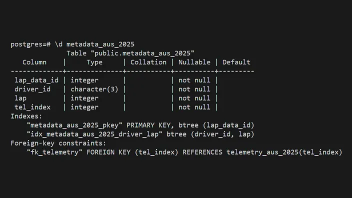
Our database has 2 tables per race (a metadata table and a telemetry entry table).
Splitting the original 2 tables into 48 cut the rows each lookup had to scan by 24x, and a B-tree index on driver and lap then made lap queries roughly 10x faster (based on my notes at the time rather than a formal benchmark).
Our metadata table was built so we wouldn’t have to search massive telemetry tables during lookups. Each metadata row points to its sample in the telemetry table by a foreign key, so with the index on driver and lap, any one lap is a single indexed query.
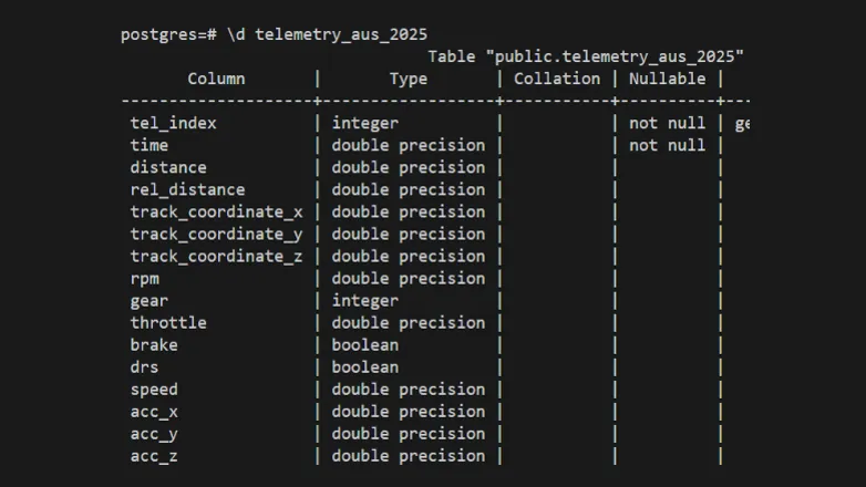
Keep in mind that telemetry is measured tens of times a second, and each of these measurements needs its own telemetry row and metadata row (over 18 million samples, so over 36 million rows across the database).
race_data.py
RaceData turns a race’s raw laps into clean and comparable data.
- Load. Every lap for every driver is fetched from the database in lap order.
- Align by distance, not time. Each lap is interpolated onto the same 500 distance points along the track for clean comparisons.
- Normalize per driver. Each of the eight metrics is scaled 0–1 against the driver’s own 2nd to 98th percentile over a block of five laps, so one spike can’t stretch the scale, and tire wear is accounted for.
- Drop outlying laps. The first lap always gets dropped, and so does any lap more than 1.5 × IQR slower than the driver’s norm (catches safety cars and pit stops).
- Reduce with PCA. The eight metrics at each point compress to ~4–5 components that account for 95% of the variance, taking a lap from 4,000 values to about 2,000–2,500. We found much better cluster results with this mechanism.
Here’s step 2, the alignment, in code:
def _reindex_df_operations(self, df):
    uniform_index = np.linspace(0, 1, DATAPOINTS_PER_LAP)
    df = df[~df.index.duplicated(keep='first')]
    df = df.reindex(df.index.union(uniform_index))
    df = df.infer_objects(copy=False)
    df = df[df.index.notna()]
    df = df.interpolate(method='index')
    df = df.ffill()
    df = df.bfill()
    df = df.reindex(np.linspace(0, 1, DATAPOINTS_PER_LAP))

    return df
kmeans_clustering.py
Each individual lap is sorted into one of five clusters, and a driver’s style is represented by a distribution across the different clusters.
Besides K-means, we looked at three other algorithms. Hierarchical clustering needs O(n2) memory, which made evaluating an entire season difficult, and the distributions it did produce were much worse. Gaussian mixtures gave the same results as K-means when using hard labels, and their real advantage, soft assignments, went against our strategy of classifying each lap into one cluster. DBSCAN never made it past planning, since it separates clusters by density and F1 laps are too alike for that to work.
Adding PCA lowered the silhouette and Davies-Bouldin scores, yet it was the first run where drivers’ distributions actually differed, so we judged every run by its distributions as well as its scores.
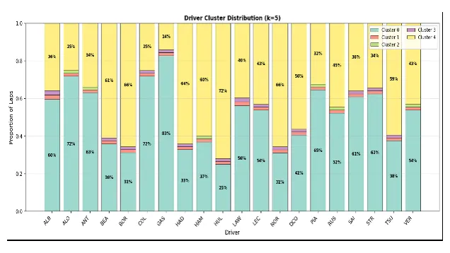
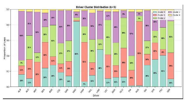
We left the clusters unlabeled. A cluster’s meaning changes from track to track, so the dashboard shows how each one differs from the race average and leaves the interpretation to the user.
Architecture
Our pipeline had three layers. This diagram displays the path from raw telemetry to the dashboard.
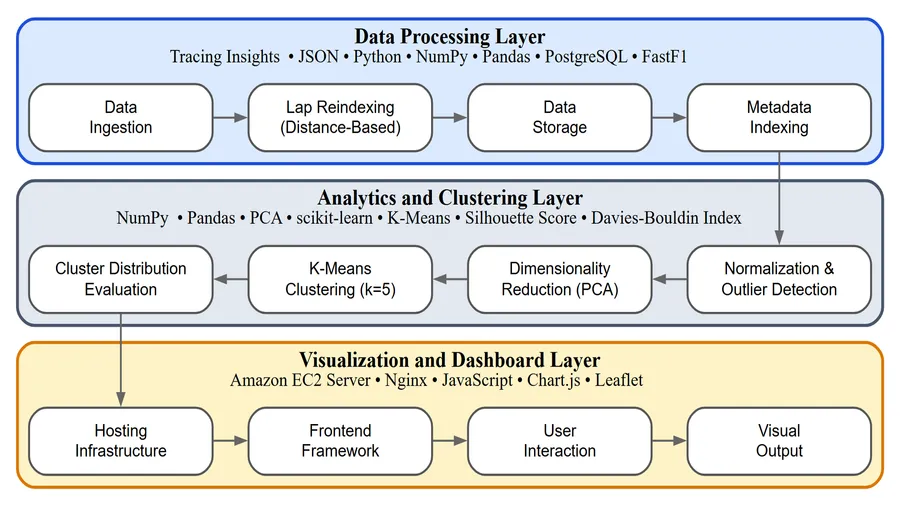
We hosted this on an EC2 instance during the capstone, but now I self-host it.
What I'd do next
Three things I would add if we had more time.
- More seasons. Covering 2025 alone limits race-to-race comparisons. More years would show how a track evolves over time, and give us more data to compare drivers by.
- Style beside performance. Adding performance metrics like lap time, pace, and finishing position to each cluster would let a user compare how a style was driven versus how well it actually did, without leaving the dashboard.
- Findings from the tool. Building it took the whole year, and none of us were data scientists, so we never used it to answer any style questions ourselves. The next step is the analysis, such as which styles are fastest, how a style changes as tires wear, and what separates two drivers in the same car.
Awards
-
1st Place, CSCE Undergraduate Enrichment Fund ($1,000)
Recognized for outstanding capstone project work by the Department of Computer Science and Computer Engineering. Presented by our capstone professor Dr. Patitz, with the award stewarded by Dr. Ogden. -
1st Place, College of Engineering Expo (CSCE)
Earned first place among Computer Science and Computer Engineering teams for our Formula 1 telemetry analysis and visualization project. -
Invited Presenter, CSCE Alumni Conference
Selected as one of three capstone teams invited to present our project to University of Arkansas CSCE alumni.

Next stop: Satellite Particle Filter
or